3. RStudio Data Processing
In this second part, we’ll perform some basic processing on some synthetic forest inventory data.
3.1. Load external data into R
The most straightforward way to load data into R is to use comma-separated values (.csv) format, a text file format that separates records across rows and fields with commas. CSV files can be exported from spreadsheet software (e.g. Microsoft Excel).
The .csv file we’ll use is named plot_data.csv, and can be downloaded here.
Save plot_data.csv somewhere memorable (e.g. Desktop). You can open this file with a text editor (e.g. Notepad) or as a spreadsheet (e.g. Microsoft Excel) if you’d like to take a look at its contents.
This file contains synthetic data for 25 forest plots in miombo woodlands each sized 50 x 50 m (0.25 ha). Each row contains data for a unique stem, where stems have a range of properties (e.g. DBH, height, species, etc.).
Attention
The data we’ll use in this exercise is entirely made up. Definitely don’t use this dataset for any quantitative work!
To load the data into R, we’ll need two commands. First, we’ll need to set the ‘working directory’, which is the location that R will run and where we will reference the CSV file relative to.
Set the working directory to the location you saved the data to as follows:
> setwd('C:/Users/your_username/Desktop/')
Note
- Make your you replace
your_usernamewith your actual username. - Note that the directory is referenced with
/rather than\, this is because\has a special meaning in R. - If you saved
plot_data.csvat any location other than the Desktop, you’ll need to reference that location instead.
To load the data into R, you can use the read.csv() function, as follows. Be careful with inverted commas, and don’t worry for now about what stringsAsFactors = FALSE means:
> df <- read.csv('plot_data.csv', stringsAsFactors = FALSE)
Once you’ve successfully loaded in the data, you can take a peek at the first few lines of it using the head() command:
> head(df)
plot_code tag_id                  species  DBH height status x_location y_location
1   plot_01   A001  Parinari curatellifolia  9.8   12.0  alive        1.2        1.9
2   plot_01   A002       Terminalia sericea 44.9   24.0  alive        4.3        3.4
3   plot_01   A003       Afzelia quanzensis  6.3    8.5  alive        1.6        3.8
4   plot_01   A004  Erythrophleum africanum 16.9   20.0  alive        2.0        4.6
5   plot_01   A005       Terminalia sericea  9.9    9.0  alive        0.1        7.5
6   plot_01   A006 Brachystegia spiciformis 30.7   22.0  alive        3.1        8.3
Don’t go any further until you’ve been able to replicate the output above.
3.2. Data frames
What you’ve loaded in is callled a ‘data frame’. Data frames are a format that store data like a table. The top line of the table is called the header, and contains the name of each column, and following rows denote data points. In this case, columns contain a range of properties of trees (species, DBH, height, etc.), and rows contains data for an individual stem.
Data frames can contain multiple types of data, but each column of a data frame has to be a single type. For example, in this case the column plot_code is a character, and DBH is a numeric data type.
Individual columns of the data frame can be accessed using the $ operator, which returns a vector. For example:
> df$DBH
[1]  9.8 44.9  6.3 16.9  9.9 30.7  6.9  9.1  6.9 20.6 28.7 45.8  5.7 12.8  9.7 20.7  8.9 13.5  5.5  5.5  6.2 10.3 27.9
[24]  6.1 36.7 19.2  5.5  8.5  5.6 38.6 17.2 17.3  9.1 24.3 12.4 13.0 15.9 16.4  8.2  6.2  7.0 31.4  6.1 41.5  8.0 28.0
[47]  6.3 85.6  8.2 53.5 37.7  9.8 16.7 13.3 10.0  6.6 19.2 11.9  9.2 14.1  8.0 10.0 23.3  9.6  5.3 18.4 27.0 23.8 71.4
[70] 13.0 52.1 13.8 23.6  6.4 11.9 13.4 10.6 44.2  7.5 10.6 44.5 11.1 13.9 24.5 25.0  7.2  8.9 42.1 13.1 17.7 19.7 19.0
[93] 21.8 22.0  9.7 23.6  8.1 15.0  5.6 23.7 15.9 21.5  8.2  8.6 14.9  7.7 13.5 12.1  5.8  6.8 15.5 83.2  6.9 35.6  8.4
[116]  6.4  9.7 22.8 16.8 12.8  5.8 29.0  5.8 14.0  5.2 12.8 10.6 17.7  8.0 23.4 31.4 26.2 17.7 18.7  7.1 11.5 29.5  7.4
[139]  9.3 13.0 11.4 18.1 49.7  6.7  5.9 23.4  7.9  5.4  6.3  7.1 13.8 27.6 13.6  9.7 16.1  5.0 48.0 26.0  6.1  6.7 17.3
[162] 19.0 12.3 21.6  5.0 16.5 28.2 22.3 18.5 17.4 31.6 23.7  8.0 22.5 14.6 19.5 13.8 74.2 13.7 24.7 18.0 10.8 11.4 30.3
[185] 11.2 17.8 38.4  9.4 32.1 16.9 19.4 11.6 17.1 35.3  6.5 28.6 11.5 38.6 15.9  7.5  9.2 40.8 11.5  8.9 22.1 12.3 35.2
[208] 27.3 20.7 21.3  7.1  5.4  7.9 16.6 31.0  6.0 30.3  9.4 26.8 19.9 22.4 22.1 49.0 13.6 28.1 28.8  6.5  9.9 23.2 21.4
[231] 19.6 49.0 11.1 25.4 14.2 10.2  9.4  5.8 38.1 33.1 11.1 16.1 17.1 15.5 19.5  7.8 20.5 28.0 29.3  9.1 44.0 24.3 42.3
[254]  9.2 15.7  7.2 16.1 44.2 18.2 15.9 34.4  5.5  7.5 12.2 11.4  7.8 20.1 39.7  6.3 10.8  9.1  6.9  8.2  5.3 11.1 14.4
[277] 31.7  5.6 20.5 16.3  5.4 12.0  7.4 19.5 16.4 27.9 15.6 22.9 57.1 15.4  6.5 13.0 33.0  7.9  8.9 19.6 12.4 20.1 16.7
[300]  6.7  5.9 12.4 23.5  9.5 13.8  5.4 40.9 22.0 31.0 19.8  6.7 41.4 42.1  5.9 30.9 20.9 40.4  6.5  8.1  8.2 14.9 15.2
[323]  7.4 19.1 18.6 10.1 18.1 19.2 44.7 41.4  7.4  5.3 22.2 19.7 10.6 39.2 20.7  8.1 15.2 12.8  7.9  6.1 27.1 19.4 15.2
[346] 16.0 44.5 20.3  8.1 47.8 11.1 11.6 11.4 18.6 25.1 10.4  5.5  9.1  8.7  7.3 12.2 26.8 25.2 17.8  9.2 11.6 11.9 24.0
[369] 12.8 18.9  9.0 11.4  9.5  9.4  7.7  7.6  6.9  5.2 10.6  7.9  7.0 18.9 25.4 15.7 11.9 26.6 48.3 11.4  5.2 24.0 19.4
[392] 10.4 24.4 36.4 10.7  7.4  7.5  7.8 23.1 21.1 15.7 16.8 23.0 10.1 33.0  5.7  9.5 24.6  5.4  5.6 21.9 27.6 15.9  6.6
[415]  5.0 17.5 20.3  6.5 12.1 13.6 20.6  9.4  9.4  8.5 13.6  7.4 10.0 10.0 11.6 14.8 14.4 13.7  5.9 55.1  7.9 11.1 35.6
[438] 12.8 32.6 19.7 16.2 13.3  9.7 15.1 53.9 28.1 22.3  9.1 13.8 12.5 35.0  6.6 33.0 10.0  8.1 31.0 18.6 57.8  9.0  5.2
[461] 11.1 46.2 11.2 30.1  8.3 11.9  7.8 37.7  9.9 23.3 23.8 12.9  5.9  8.5  7.7 18.2  5.6  5.4  5.4 30.5 18.2 11.9  8.8
[484] 30.1 20.1 15.3  6.7  6.6 18.6 17.2  5.4 14.6 15.7 16.1 31.9 42.2  8.2 25.7 20.0  9.4 23.1 18.2 22.0  8.7 12.2 35.4
[507] 17.6  7.0 11.5  6.7 13.1  5.2  6.6 19.4 12.8 13.8 32.2 16.3 17.3  6.9 59.2 15.5 11.5 22.4 32.5 17.5 15.6 13.1  9.6
[530] 10.0  9.5 57.9 26.1  6.7 18.6  5.3 15.0  8.1 20.9 39.3 15.4  6.1 15.9  6.5  7.5 13.7 30.7 28.0 44.0  8.2 12.5 12.5
[553] 19.1 30.7 28.1 12.5  8.3 34.7  8.4 81.8 60.6 17.3 14.1 20.4  9.2  6.2 16.4 27.4 13.4 18.2 20.7 36.9 34.9  6.4 51.2
[576] 11.1  5.2  7.2 43.8 19.1 45.5 17.2 16.6 21.7 23.8  5.0 28.1  6.0 11.1 16.8 14.5  5.4 16.2 10.7 17.4 28.3 19.4 43.6
[599] 27.5 12.7 16.3  9.8 13.4 24.6 18.5 38.6  7.4 15.4  5.2 11.4 33.2 32.9 12.8 31.9  7.7  6.9 13.6 10.7  7.3  7.0  9.9
[622]  5.5 15.8 37.9  7.9  6.4 49.0  9.3 33.6  5.7  6.5 52.6  8.5  5.1  6.8 12.0 10.8 24.3  9.6  5.9  5.4 30.6 28.8 30.9
[645]  7.0 24.8  5.4  9.9 21.5 16.3  6.0  9.6 25.9 17.3  6.9 32.7 18.3  6.7 22.9  6.9 14.2  9.9 26.6 50.8 12.8 20.5 38.5
[668] 13.8  5.9 23.0 14.4 20.0 35.4  9.1 65.5 43.6 11.6 29.9  6.0 25.7 40.9  8.9 19.1 15.3 13.8 33.3 11.1  5.9 12.7 11.1
[691]  7.1  7.2 10.7  7.4  6.8 10.3 13.7 14.2 22.8 33.7  6.2 12.9  7.3 35.0  8.9  6.5 25.1 20.2  5.4  8.5  9.3  7.9  7.5
[714] 21.6 18.4  5.9 14.4 50.7 60.3 16.7  7.9 10.2 15.4  6.4 11.7 11.8 17.8  9.2 11.1  7.8 19.4 30.8 14.9  7.5 36.6 66.8
[737]  8.7 38.7  5.4 12.1  9.8  9.7 10.8 40.3 10.0 23.4  5.4 36.2 10.4  7.4  6.3 16.6  7.6 24.8 66.4 16.4 12.1 30.9  9.9
[760]  8.6  9.5 10.3 20.9 12.0 15.8  9.3  8.9 21.2  8.9 52.4  7.8  6.6  5.8  6.2 11.5  6.8 22.8 39.2 20.0  8.0 16.5  6.4
[783] 12.0 16.5 19.6 13.5 15.6 12.6 19.9 19.5 20.7 17.2  6.6 25.8  7.9 10.4  6.6 12.1 10.1 31.9 31.9 11.2  8.1 26.9  6.8
[806] 11.3 18.2  5.6 11.5  8.8 13.6  8.1  9.0 15.8 10.3 30.4 24.5  9.1 12.3  9.5 19.0 35.9 15.3 24.2  6.6 23.7 15.0  6.8
[829] 19.4 15.2 21.3 27.1 33.6 14.9  6.4 19.1  5.5 89.0  5.6 10.2 85.1  6.6 10.1 10.0 10.3 19.4 11.0 17.2 20.6  5.7 19.9
[852] 32.7  5.5 19.5 17.4 12.8 37.1 11.7 34.6 12.6 57.7 27.3  5.2  5.8 12.2 14.7 23.5 25.8 30.6 20.5 23.0 15.4 26.0  7.0
[875] 11.2 14.2 10.0 26.3 38.0  9.1  9.3  6.8 15.4  7.6 14.9  5.9 22.6 32.7  5.2 10.0 12.4 13.6 32.6 16.4  8.8 12.2 55.3
[898] 12.2 63.4 20.5  6.0 21.3 41.3 34.9 17.4  5.9 11.4 15.5  9.9  9.7 19.2 16.6 10.8 10.6 47.6 12.4 24.2 16.3 29.6 16.1
[921]  5.7  7.3  8.7 14.2 53.5  8.5 53.8  9.6 15.8  6.1  9.7 10.1  5.8 64.5 11.0 40.3 12.7  6.9 15.3 14.7 39.8 20.4 19.9
[944] 21.3  7.9 27.9  7.5 14.0 19.3 26.5 16.5  5.7 15.6 22.0  7.9 12.7  6.2 23.4  8.8 26.8 27.1 48.6 21.7 16.3  5.5 14.7
[967]  6.7 17.4 45.7 45.7 23.9 16.0  7.3 10.9 43.9 13.3  8.2 44.1  6.5  7.3 12.8  9.7 12.6 21.5 27.5  9.8  7.0 22.3  5.2
[990] 19.0 15.1 12.1 14.3  6.8 14.7  7.8  5.3 11.6 13.0  5.4
[ reached getOption("max.print") -- omitted 2580 entries ]
3.2.1. Exercises
Now it’s your turn!
- Calculate the mean average DBH in this dataset (HINT: recall the
mean()function. - Try to extract a vector of species names from the data frame.
3.3. Generating statistics
Often we’ll want to summarise our data rather than view a raw vector of numbers. A good way to do this is with the summary() function, which returns key statistics for each column of a data frame:
> summary(df)
plot_code            tag_id            species               DBH           height         status            x_location      y_location
Length:3580        Length:3580        Length:3580        Min.   : 5.0   Min.   : 2.50   Length:3580        Min.   : 0.00   Min.   : 0.00
Class :character   Class :character   Class :character   1st Qu.: 8.4   1st Qu.:10.50   Class :character   1st Qu.:12.68   1st Qu.:11.88
Mode  :character   Mode  :character   Mode  :character   Median :13.6   Median :16.00   Mode  :character   Median :25.40   Median :25.25
                                                        Mean   :17.5   Mean   :16.95                      Mean   :25.31   Mean   :25.04
                                                        3rd Qu.:22.4   3rd Qu.:22.00                      3rd Qu.:38.10   3rd Qu.:37.80
                                                        Max.   :92.9   Max.   :57.50                      Max.   :50.00   Max.   :50.00
We can also apply summary() to an individual column of a dataframe:
> summary(df$DBH)
   Min. 1st Qu.  Median    Mean 3rd Qu.    Max.
    5.0     8.4    13.6    17.5    22.4    92.9
Other individual statistics can be calculated with built-in R functions, for example:
> mean(df$DBH)
[1] 17.50045

> median(df$DBH)
[1] 13.6

> sd(df$DBH) # Standard deviation
[1] 12.38198

> max(df$DBH)
[1] 92.9
When looking at character data, we can use other forms of summarising data. For example:
> unique(df$plot_code) # Return unique plot values
[1] "plot_01" "plot_02" "plot_03" "plot_04" "plot_05" "plot_06" "plot_07" "plot_08" "plot_09" "plot_10" "plot_11" "plot_12" "plot_13" "plot_14" "plot_15"
[16] "plot_16" "plot_17" "plot_18" "plot_19" "plot_20" "plot_21" "plot_22" "plot_23" "plot_24" "plot_25"

> table(df$plot_code) # Return number of stems in each plot
    plot_01 plot_02 plot_03 plot_04 plot_05 plot_06 plot_07 plot_08 plot_09 plot_10 plot_11 plot_12 plot_13 plot_14 plot_15 plot_16 plot_17 plot_18 plot_19 plot_20
    159     120     233     263     165     154     188      93     139      46     229     192      33     117     256      70     204     135     199     206
plot_21 plot_22 plot_23 plot_24 plot_25
    70     108      56      73      72
R also lets us modify and create new columns. Let’s say that we wanted to calculate DBH (currently in units of cm) in metres and save it to a new column:
> df$DBH_m <- df$DBH / 100

> summary(df$DBH_m)
    Min. 1st Qu.  Median    Mean 3rd Qu.    Max.
0.050   0.084   0.136   0.175   0.224   0.929
We can this new column to calculate basal area, which is usually expressed in units of m^2:
> df$basal_area <- pi * (df$DBH_m / 2) ** 2    # pi * r^2

> summary(df$basal_area)
    Min.  1st Qu.   Median     Mean  3rd Qu.     Max.
0.001963 0.005542 0.014527 0.036092 0.039408 0.677831
3.3.1. Exercises
- What is the mean and standard deviation of tree heights in the entire dataset?
- How many different species are there in this dataset?
- What are the three most common species in the dataset?
- Can you figure out what was the minimum DBH measured in these plots?
3.4. Aggregation
We often need to aggregate stem data to plot summaries. This is where using R in place of spreadsheet software starts to become very powerful.
Let’s use the basal_area column we defined earlier to calculate the total basal area of each plot. To sum the basal area in each plot we can use the aggregate() function. Be careful here, the syntax of this function differs from what we’ve covered already.
> df_plot <- aggregate(basal_area ~ plot_code, df, sum)

> df_plot$basal_area <- df_plot$basal_area / 0.25 # Translate to units of m^2/ha, as our plots are 0.25 ha in size

> df_plot
plot_code basal_area
1    plot_01  25.084091
2    plot_02  19.177783
3    plot_03  30.126482
4    plot_04  43.599101
5    plot_05  27.744608
6    plot_06  21.809257
7    plot_07  28.908511
8    plot_08  12.148756
9    plot_09  18.025749
10   plot_10   6.285862
11   plot_11  31.490451
12   plot_12  24.466042
13   plot_13   6.756331
14   plot_14  14.503772
15   plot_15  33.763903
16   plot_16   9.690883
17   plot_17  29.543069
18   plot_18  19.004022
19   plot_19  28.991242
20   plot_20  31.032360
21   plot_21   9.942044
22   plot_22  14.048863
23   plot_23  14.682639
24   plot_24   8.452713
25   plot_25   7.557422
The aggregate function produced a new data frame, where instead of each row being an individual stem each row instead relates to a plot. We can run this new data frame through some of the functions we’ve already learned. For example:
> summary(df_plot$basal_area)
 Min. 1st Qu.  Median    Mean 3rd Qu.    Max.
 6.286  12.149  19.178  20.673  28.991  43.599

> mean(df_plot$basal_area)
 [1] 20.67344
We can substitute the sum part of the aggregate function for another statistic. For example, to calculate stocking density, we might use:
> df_sd <- aggregate(tag_id ~ plot_code, df, length) # Calculate number of unique tags
We can combine this with our already made plot scale dataframe by adding a new column to df_plot:
> df_plot$stocking_density <- df_sd$tag_id
3.4.1. Exercise
Instead of by plot, try to aggregate the data by species. Use the data frame you produce to figure out:
- What is the average basal area of each species? What are the dominant species in this dataset?
- What species has the lowest total basal area?
3.5. Making plots
R is also very well suited to making publication quality plots. We can produce plots with the plot command. For example:
plot(height ~ DBH, df)
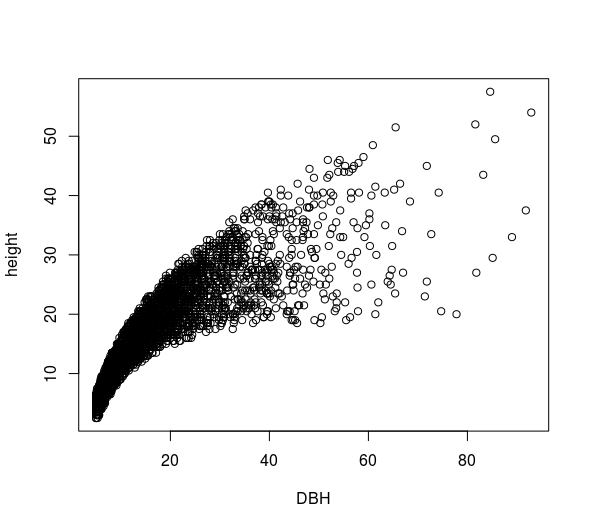
This plot shows a positive relationship between DBH and stem height, as might be expected.
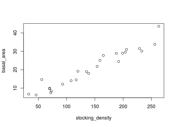
3.5.1. Exercise
- Using
`df_plot, can you build a plot of stocking density vs basal area? The resulting plot should look something like this:
3.6. Overview
Well done! Again, don’t worry if it didn’t all make sense, programming takes a long time to understand.
Here you’ve been introduced to data analysis in R. You should now understand:
- How to load data into R (i.e.
read.csv). - How to use and manipulate data frames (e.g. the
$operator). - How to generate summary statistics with data frams (e.g.
summary). - How to aggreate data (i.e.
aggregate). - How to make simple plots using data (i.e.
plot).
3.7. Further reading
If you want to continue learning R, we can recommend the following resources:
- https://www.datacamp.com/courses/free-introduction-to-r
- https://www.youtube.com/playlist?list=PL6gx4Cwl9DGCzVMGCPi1kwvABu7eWv08P
- https://ourcodingclub.github.io/
- https://r4ds.had.co.nz/
Happy coding!