2. RStudio 101

Welcome to R!

R is a relatively straightforward programming language commonly used for data processing and alaysis. It’s open source, freely available, and very widely-used in scientific fields, including in ecology and forestry. It’s also relatively easy to pick up, so it’s a great place to start to learn programming.

2.1. RStudio Layout

RStudio should look something like the following:

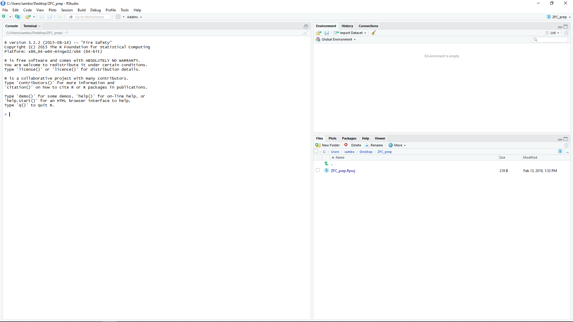
The important part of RStudio for this tutorial is the Console window, located on the left (or bottom-left) of RStudio. In this window you can run R ‘interactively’, which allows you to run R commands on-the-fly, and receive immediate answers.

In the workshop we’ll be using a combination of ‘interactive’ programming and writing scripts, but for the following tasks, we’ll work in the ‘interactive’ mode only. Commands can be typed following the > symbol, and submitted by pressing ‘Enter’.

2.2. Commands

Write the following command in the console window, and submit it with Enter. Be very careful to copy it exactly, including the inverted commas.

> print('Hello World!')

If the command has worked, you should see:

> print('Hello World!')
[1] "Hello World!"

If instead you got an error, double-check that you copied the phrase precisely.

What has happened here is that you’ve instructed R to print a phrase to the terminal. The phrase Hello World! was written to the terminal after the command.

Practice using the print function in R until you’re familiar with it:

> print('I can get R to print anything I type')
[1] "I can get R to print anything I type"

> print('Even numbers like 6 and symbols like #')
[1] "Even numbers like 6 and symbols like #"

There are hundreds of other commands available in R (commonly known as ‘functions’). What do you think the following functiuons do?:

> toupper('Hello World!')
[1] "HELLO WORLD!"

> nchar('Hello World!')
[1] 12

> paste('Hello', 'World!')
[1] "Hello World!"

Tip

You can access help for R functions using a ? symbol in the console window. For example: ?print, ?toupper etc. This will bring up a text description of how the function works, and what inputs it requires.

2.2.1. An aside: Comments

Comments are important aspects of programs. Comments are used to describe what your program does in readable language, or to temporarily remove lines from a program. Comments are indicated by the # symbol, and anything that follows won’t be executed.

We’ll now use comments to describe the code. Adding comments to your code is good practice as it makes your code easier for other people to use, and helps you to remember how your own code works. For the purposes of this tutorial, you won’t need to copy out anything after the # symbol.

2.3. Calculations

Until now you’ve been working with letters and symbols, a data type in R known as characters. R is also able to handle numbers, which are represented by the data types named integer (for whole numbers) and numeric (for numbers with a decimal point.

Attention

Unlike characters, integer and numeric data types are not surrounded by inverted commas.

We can use R like a calculator to perform arthimetic on numbers. Try the following:

> 1 + 2 # Addition
[1] 3

> 1 - 2 # Subtraction
[1] -1

> 3 * 4 # Multiplication
[1] 12

> 5 / 2 # Division
[1] 2.5

We can also use R to peform more complex operations:

> 8 ^ 2 # Power functions
[1] 64

> log(10) # Natural logarithm
[1] 2.302585

> pi # Access constants
[1] 3.141593

2.4. Variables

In programming, variables are names that we give for something. They ensure that code is readable, and offer a means of ‘saving’ a value for later use. We assign a value to a variable in R either using the = or <- symbols, with the variable name on the left and it’s value on the right. Try these examples of how variables work:

> x <- 1

> x
[1] 1

> y <- 1 + 2

> y
[1] 3

> z <- x + y

> z
[1] 4

2.4.1. Exercises

1. Use the +, -, *, and - operators to compute the following:

   • 123456 plus 654321
   • 123456 minus 654321
   • 123456 multiplied by 654321
   • 123456 divided by 654321
   • 123456 squared

2. The basal area of a tree (BA) can be calculated using the equation:

   • BA = π(DBH/2)^2

…where DBH is the tree diameter at breast height and π = 3.14. Use R to calculate the basal area of a tree of 50 cm DBH.

2.5. Logical data

Logical data can take two values; TRUE or FALSE (sometimes denoted as 1 or 0). The logical data type is most commonly associated with logical expressions. The main logical expressions we use in R are as follows:

> # An equivalence statement tests whether two arguments have the same value.

> 1 == 1
[1] TRUE

> 1 == 2
[1] FALSE

> FALSE == FALSE
[1] TRUE

> TRUE == FALSE
[1] FALSE

> # A negation statement tests is the opposite of an equivalence statement.

> 1 != 2
[1] TRUE

> 1 != 1
[1] FALSE

> TRUE != TRUE
[1] FALSE

> FALSE != TRUE
[1] TRUE

We can combine logical statements together:

> # The '&' statement (conjunction) returns TRUE where both arguments are TRUE.

> 1 == 1 & 2 == 2
[1] TRUE

> TRUE & TRUE
[1] TRUE

> TRUE & FALSE
[1] FALSE

> FALSE & FALSE
[1] FALSE

> # The '|' statement (disjunction) returns TRUE where either of the arguments is TRUE.

> 1 == 2 | 2 == 2
[1] TRUE

> FALSE | TRUE
[1] TRUE

> FALSE | FALSE
[1] FALSE

> TRUE | TRUE
[1] TRUE

Logical statements like these may be quite different from anything you’ve learned before, so don’t worry if this is still confusing!

2.6. Groups of things

Frequently we will want to group multiple values together in a single variable. The main mechanisms for doing this in R are vectors, lists and data.frames. Here we’ll focus on vectors and later dataframes, but you should be aware that many methods exist of grouping in R.

2.6.1. Creating vectors

Vectors are a group of ordered elements. They are created as follows:

> my_vector <- c(2, 4, 6, 8) # Use the command c() to define a vector, separating elements using commas

> my_vector
[1] 2 4 6 8

>>> my_vector <- c(my_vector, 10) # Add a new element to the end of a vector

>>> my_vector
[1] 2 4 6 8 10

2.6.2. Exercises

1. Try to create your own vector containing the letters ‘A’ to ‘F’
2. Append the letter ‘G’ to the end of your vector

2.6.3. Indexing vectors

We can access individual elements of a list using indexing. We do this using square brackets and specifying the numeric location of the elements we want to access.

Here are some examples of how we index vectors:

> zoo <- c('Tiger', 'Parrot', 'Bear', 'Sloth', 'Giraffe') # A list of animals in a zoo

> zoo[1] # Get the first element of the list
[1] "Tiger"

> zoo[4] # Get the fourth element of the list
[1] "Sloth"

2.6.4. Modifying vectors

We can also modify vectors, as follows:

> zoo[2:4] # Get the second to fourth elements from the vector
[1] "Parrot" "Bear"   "Sloth"

> rev(zoo) # Reverse the vector
[1] "Giraffe" "Sloth"   "Bear"    "Parrot"  "Tiger"

> zoo_reverse <- rev(zoo) # We can 'save' the change by declaring a variable

> zoo_reverse[3] <- "Lion" # Modify the third element of the list
> zoo_reverse
[1] "Giraffe" "Sloth"   "Lion"    "Parrot"  "Tiger"

2.6.5. Vector functions

We can determine various properties of vectors using the following functions:

> my_vector <- c(2, 4, 6, 8, 10)

> min(my_vector) # Returns the minimum value of a vector
[1] 2

> max(my_vector) # Returns the maximum value of a vector
[1] 10

> length(my_vector) # Returns the number of elements (length) of a vector
[1] 5

We can also pefrom standard mathematical operations on vectors. For example:

> sum(my_vector)
[1] 30

> my_vector / 2
[1] 1 2 3 4 5

2.6.6. Exercises:

1. Define a new vector with the numbers 1 to 10. What is the sum total of this vector? Can you reverse it to count from 10 to 1?
2. Can you figure out how to calculate the mean average and standard deviation of my_vector as defined above? HINT: Google is your friend!

2.7. Overview

Congratulations for reaching this far, learning to program is hard work! Don’t worry if you didn’t catch everything, we’ll be going over much of this again in the workshop.

Here you’ve been introduced to some of the basic operations in R. You should now understand:

1. How to use functions (e.g. print(), length(), rev()).
2. Definition and use of variables.
3. Performance of basic arithmetic (e.g. +, -, *, /).
4. How boolean logic works in R (i.e. TRUE, FALSE).
5. How to use vectors to store multiple values together (e.g. c(1,2,3)), access individual elements of vectors, and perform mathematical operations on all values of a vector.

In the remainder of this introduction to R we’ll load some synthetic forest inventory data in R, perform basic statistical analyses, and learn to draw plots.